22/01/2026 11:59 AM - Lecture
22/01/2026 11:59 AM - Lecture
Still on Lecture 4
Same lecture as last starting from policy iteration
Finite number of iterations to get optimal policy yada yada.
Each iteration guarantees improvement to the value function
This must be difficult to prove
After the value function converges the policy may change once more, but both final policies are equivalent in terms of value so either can be chosen.
These were both model based algorithms (Know the average reward for taking an action and the conditional transition probabilities) that only apply with finite state spaces and action spaces. When the model is not known we need to learn that as well.
Q-Learning
Lecture 5
Off-policy model free algorithm.
(Different than online and offline)
Define a Q function $Q(i, u)$ (action value function) as the expected value of the sum of future rewards after taking the action from the state.
$$
\begin{align}
Q(i, u) &= E(r(i, u) + \alpha V^(j)) \
&= \bar{r}(i, u) + \alpha \sum_j P_{ij}V^(j)
\end{align}
$$
where $j$ is the distribution over the future state given the action.
This is the exact form of the equation we use to choose the action after we have the value function. So we select $u$ as
$$
\mu(i) = argmax_u Q(i, u)
$$
Note that if we have the Q function we don't need the transition probabilities. But then the question becomes how do we get the Q function without knowing the transition probabilities? Monte carlo.
So even though there is a 1-to-1 mapping between Q and V, it is often better to learn Q.
Q-Learning
Given an experience (current state i, current action, u, reward we got r(i, u), and next state j) then we can update our estimate of the Q value.
(Only markovian models and not partially observable)
Note that Q learning also works with finite action space infinite state space when we move to deep Q learning
$$
Q(i, u) \leftarrow (1-\beta_k)Q(i, u) + \beta_k(r(i, u) + \alpha\cdot max_v Q(j, v))
$$
First term is old estimate and second term is new estimate.
$V^*(j) = max_v Q(j, v)$
$$Q(i, j) = \bar{r}(i, u) + \alpha \sum_k P_{ij}(u) V^* (j) = \bar{r}(i, u) + \alpha \sum_k P_{ij}(u) max_v Q(j, v)$$
in the perfect case and we know
$$r(i, u) + \alpha\cdot max_v Q(j, v)$$
equals this in expectation
Why not just collect many examples of taking random actions and rewards from many states and then compute the Q directly using averages? Just because we are in practice playing out games to collect experiences?
Good question: This is off-policy meaning that if we just see experiences generated from any policy we can learn the optimal policy as long as the generating policy provides enough coverage for each state (all state action pairs must be seen infinite times).
The betas must decay to 0. In practice we use a standard scheduler.
Another form we can do
$$
Q(i, u) \leftarrow Q(i, u) + \beta_k (r(i, u) + \alpha \cdot max_v Q (j, v) - Q(i, u))
$$
This form relates to temporal difference learning.
Offline: We just learn from a database without needing to act using the policy.
Off-Policy: Learning from different policy than we are teaching.
Actually it is unclear to me why this works. Because the monte-carlo assumption would... wait no the expectation is conditional on i and u so if we know i and u then when we do the sum it is actually definitely the distribution of the next state no matter what the policy is.
Tabular Q-Learning on paper
Write out your Q table that lists all states and action. States on x and actions on y for example.
When we get an experience we only update the specific state action pair that is the current state current action.
Our example:
$0.2 + \beta (0 + \alpha \cdot -0.5 - 0.2)$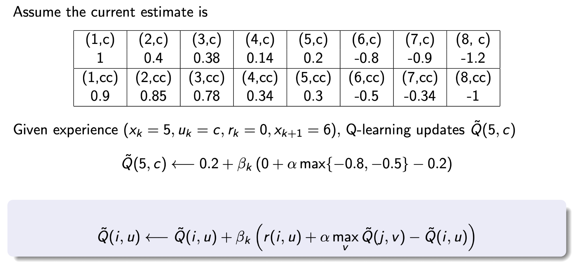
You can also use this data to learn the model and then use policy/value iteration to get the policy. However, most of the time the number of parameters you need to learn if you are learning the transition model is much larger than the parameters you need to learn if you get Q values. For learning the model in general you need to learn $S^2 A$ parameters where for Q learning it is just $SA$. Of course if you know something about the form of the problem you can collapse it down to $SA$ as well like if you know you can only transition to a fixed number of states from each other state.
SARSA
Explore the policy using an epsilon greedy search given the current Q table.
Since we know the next action we are taking this time, we don't have a max over the future Q. We just use the actual action we used.
Why is this better? The purpose of this modification is just that you don't have data. But then why not just still use the max over the future Q? Why have the epsilon for randomly selecting a different Q value than the one we curretly believe is best?
Answer: Lecturer is not sure. Converts back to off-policy. Maybe the variance in Q is useful early on when Q is very wrong?
We can also substitute epsilon greedy with softmax (Boltzman Exploration)
In both cases you need to collapse to deterministic following optimal policy at the end of training.
Off-Policy vs On-Policy
Target Policy: Policy we want to learn.
Behavior Policy: Policy that generates data.
So for example if you are learning to drive from a human driver, the human is the behavior policy and the target policy is generally the optimal policy.
Q-Learning (Off-Policy):
Target - Optimal Policy
Behavior - Any policy
SARSA (On-Policy):
Target - epsilon greedy of Q
Behavior - epsilon greedy or Q
Question: If we did what I suggested and updated the Q value with the max over the actions instead of the action we actually took, I guess the target and behavior would be different so the algorithm would be off policy? Like basically with SARSA we are learning the Q values for the epsilon greedy policy, not the optimal policy. That's why epsilon needs to go to 0 eventually. Wheras my idea learns the optimal policy directly. Maybe that breaks a proof that we converge? No it doesn't as we still always visit every state infinite times since we have an epsilon during exploration. In fact with my version we don't need epsilon to go to 0 as we visit every state action pair infinite times which is the requirement for Q-Learning to converge to the optimal policy.