ReID Pipeline
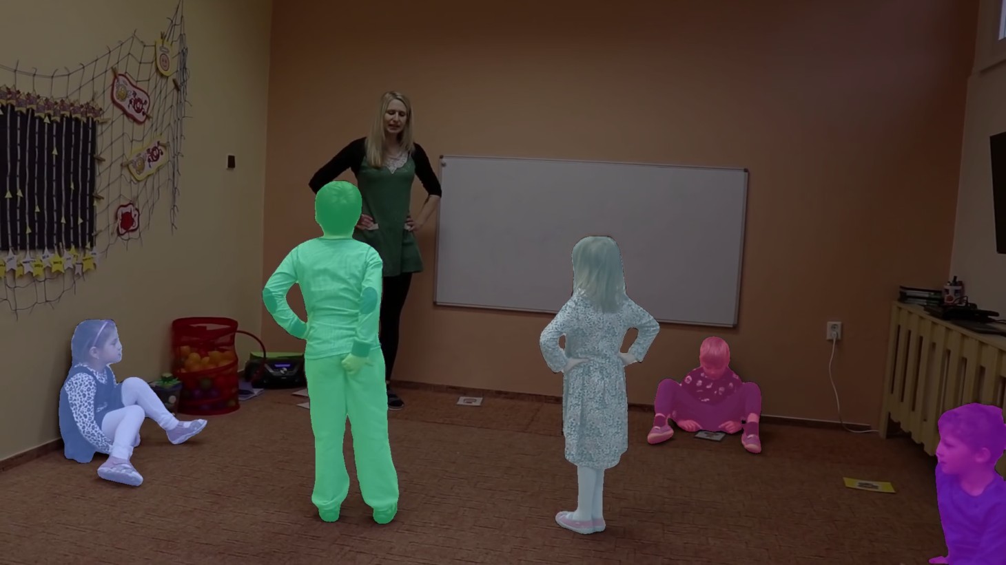
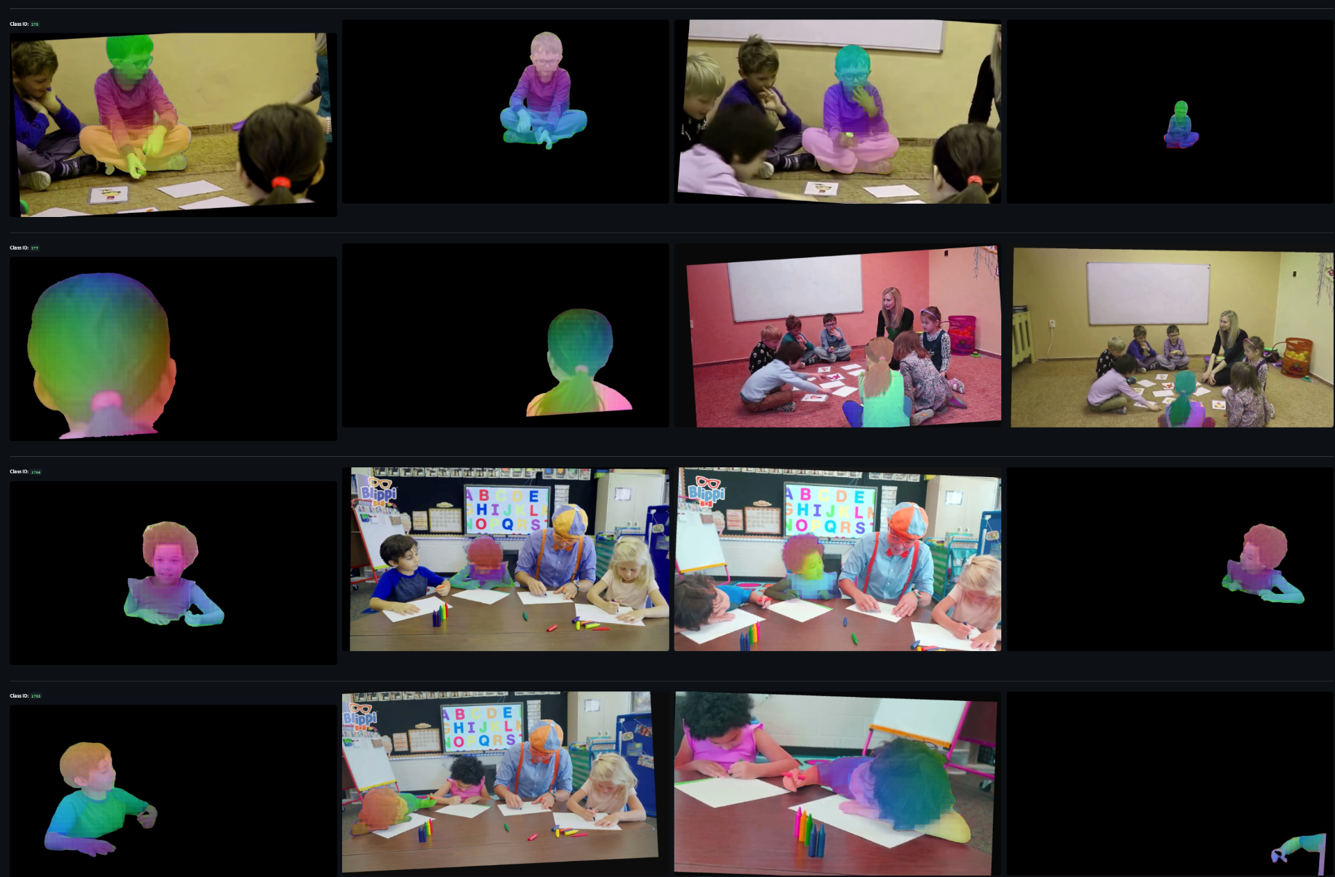
Example final segmentations -
final_reid_output.mp4 is the "masked" output where colors remain the same over the course of the video, including between cuts
raw_tracklets_output.mp4 is the raw SAM3 segmentations
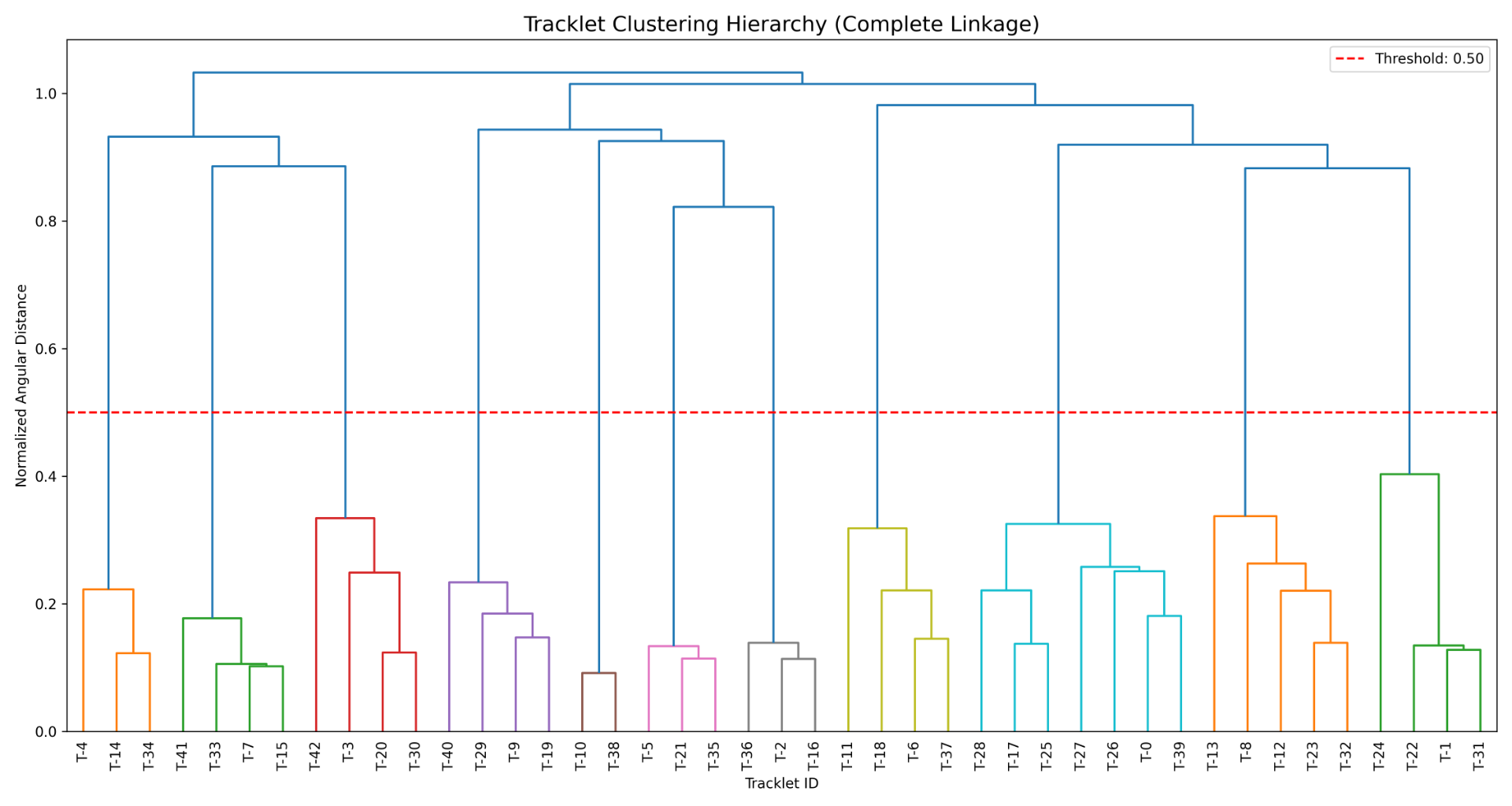
cluster_hierarchy_dendrogram.png shows how the clustering algorithm is making the decision on which tracklets to cluster.
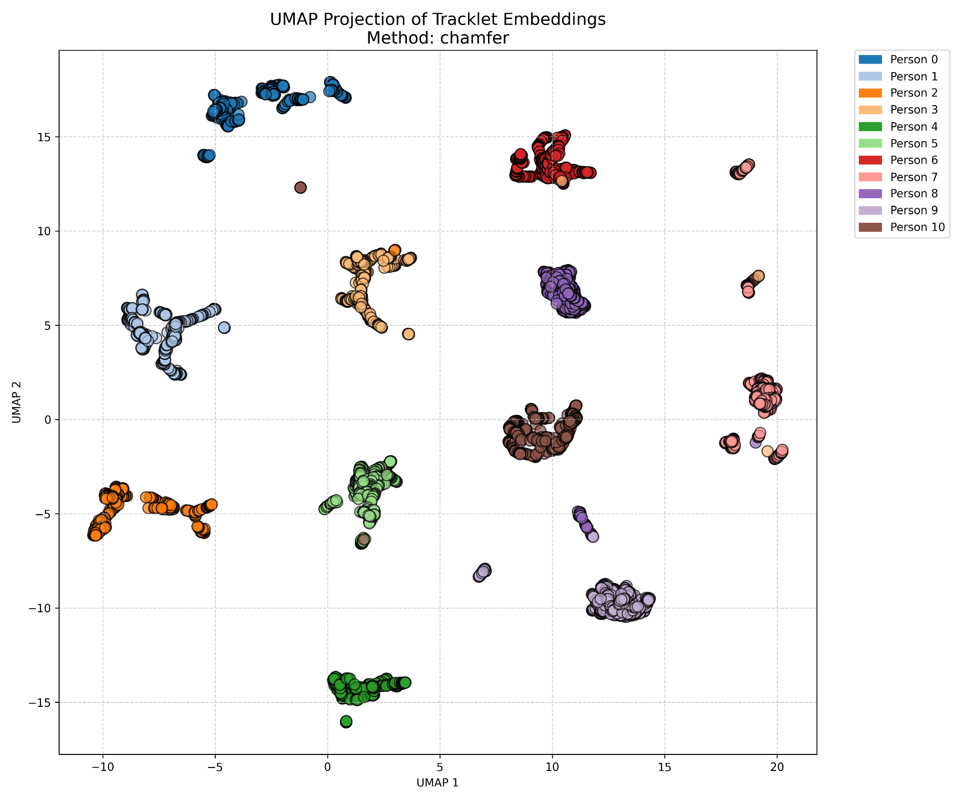
embedding_clusters_umap.png is a umap dimension reduction of all frames of all tracklets.
Easy example where we get it completely correct
Example umap clustering:
Example clustering tree:
Dataset creation
Find videos of classroom settings where students move in and out of frame and there are cuts in the video.
Cut the video into scenes by using TransNetV2 and enforce scene length less than N frames so that SAM can be run over the scene.
Segment the students with SAM in each scene.
We also pull in an external dataset Person ReID in the Wild to supplement data and increase generalization.
We then match the SAM segmentation to a set of DINO patches. The output of this is a list of DINO embeddings, one for each patch that overlaps the SAM segmentation.
Example SAM segmentation:
Example match DINO embeddings:
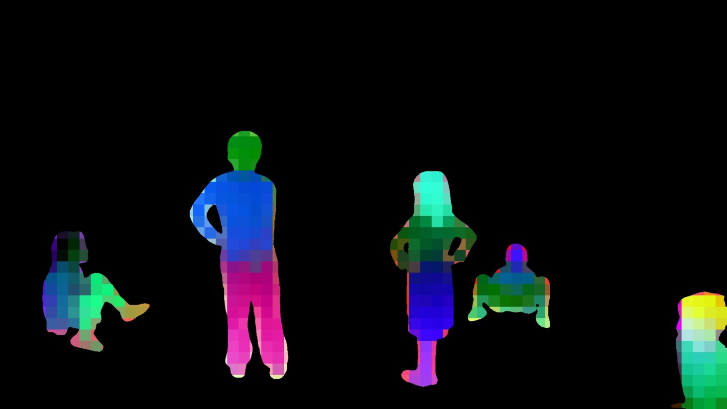
The way this was created was by matching the DINO embeddings to the SAM masks and then for each set of matched embeddings we run PCA to project down to 3 dimensions which we use for the color channels on each patch. You can see the small squares each of which corresponds to a single patch and associated embedding.
Model training
Use circle loss.
Positive set are different views of the same student within a single tracklet in a scene.
Negative set are split into two:
1. Hard negatives: Different students from the same scene.
2. Easy negatives: Any students from an entirely different video
Example of one sample from the dataset. Each row are different example of the same tracklet. The first and second row are hard negatives to each other because they come from the same scene. Same for the third and fourth. Between these two groups they are easy negatives because they come from entirely different videos.
Since we pass in a set of DINO embeddings corresponding to the patches where the student is, the model needs to be built to handle a variable input length. We tried multiple methods for this including simple averaging of embeddings, simple attention weighting, and a full transformer. The transformer performed the best to that's what we're using.
For the report, I think it would be interesting to visualize attention maps to see what parts of the student are being most attended to by the model.
Since we can generate this data from any video without manual labelling, this is a self supervised method that can be trained on any internal videos.
ReID on long videos:
The model is not trained to perform reID between scenes, but it naturally generalizes to this use case because it learned to do reID within a single scene that we hope had enough viewpoint changes of the single student to learn robust features.
1. Scene segmentation
Like when we generated the dataset, the first step is to split into scenes where viewpoint changes dramatically and by length so that SAM can process the chunks.
We also at this point extract the DINO embeddings and pass them through our contrastive model which then outputs a single embedding per student per frame.
This step outputs segmentations with matching contrastive embeddings for each student for each frame.
2. Tracklet creation
We then take the segmentations and split them into tracklets by checking when the SAM track goes fully out of frame and splitting a tracklet at that point. SAM tried to do ReID itself when a student moves out of frame and then back in, but it is unreliable so we do it ourselves.
3. Tracklet distance matrix generation
Once we have a set of tracklets that cover the entire video, we want to run our comparisons between them. For our clustering algorithm, we need to have a distance measure
Our contrastive model allows us to compare one segmentation on a single frame to another segmentation on another frame, but not one entire tracklet to another tracklet.
Note that in SOTA models they generally have a heirarchy where there is a pooling model that learns to generate an entire tracklet embedding from the individual embeddings on each frame.
For our tracklet distance measure, we first generate a tracklet similarity matrix.
Tracklet similarity matrix
We have two tracklets corresponding to two students who may or may not be the same person. Each frame in the tracklet has a corresponding embedding.
For tracklet $t \in {a, b}$, frame $f$, we denote the normalized embedding $e^t_f$.
$S_{i,j} \in \mathbb{R}^{N_a \times N_b} = e^a_i \cdot e^b_j$
$S$ is then a similarity matrix comparing each frame of one tracklet to every frame of the other.
Tracklet distance matrix
For clustering, we need to have a distance matrix instead of a similarity matrix. The most valid way to do this is using angle distance which is computed as:
$D=\frac{arccos(S)}{\pi}$
This is a valid metric in that it does things like always be above 0 and satisfy the triangle inequality.
Tracklet distance measure
$D$ defines a per-frame distance, but we need a single number to define the distance between tracklets.
SOTA uses a second network to learn a tracklet embedding that takes in the whole tracklet and outputs an embedding. We opt for a classical method.
We evaluated two distance measures:
1. p-th percentile of the flattened $D$ matrix.
2. Chamfer distance over the $D$ matrix.
The p-th percentile method is very sensitive to noise since one bad/blurry frame causes N of the entries in the matrix to become meaningless.
This can be written as $P_{90}(D)$
Chamfer distance is better because it effectively ignores bad frames by choosing to pay attention only to the frames that have the highest similarity/lowest distance.
This can be written as
$d_{\text{Chamfer-}10}(D) = P_{10}\left( \left{ \min_{1 \le j \le M} D_{i,j} \right}{i=1}^N \cup \left{ \min{1 \le i \le N} D_{i,j} \right}_{j=1}^M \right)$
We use a much lower percentile for the chamfer version as it is very robust to noise.
We end up using Chamfer-10 as our tracklet distance measure.
Upon applying this measure to all pairs of tracklets, we have a matrix $T$ where $T(i, j)$ measures the distance between tracklet $i$ and tracklet $j$.
Physical constraints
We have a hard constraint that two tracklets that overlap in time must correspond to two different unique individuals. The way we enforce this is simple. If tracklet $a$ and tracklet $b$ overlap in time, then set $T(i, j) = \infty$. This is a strong regularization for the problem.
After this we have our final distance matrix $T$.
4. Clustering
At this point we just use agllomerative clustering from scikit learn. It takes a distance matrix as input and a threshold on which to split clusters and returns labels for each of the tracklets. Each unique label is a unique individual.